Human vs computer

Image classification is the process of getting an input image and returning a class (eg: cat or dog) or a likelihood of the classes that best describe the image. For humans, recognition is one of the first skills we learn from birth and experience as effortless in adulthood. We are, unknowingly, able to quickly and seamlessly identify the environment in which we find ourselves. When we see an image, we are able to immediately characterize the scene and name each object. Unfortunately, these skills like quickly recognizing patterns, generalizing prior knowledge and adapting to different environments do not apply to computers.

What the computer sees

When a computer takes an image of a dog as an input, it sees a series of pixel values. Depending on the resolution and size of the image, the computer identifies a series of 32 x 32 x 3 numbers (assuming a 33 by 33 resolution in a typical 3 color encoding). These numbers are meaningless to humans, but are the only available input for the computer. The intention is that a computer gets a series of numbers (an image of a dog or cat) and returns percentages that describe the probability that the image belongs to a certain class (eg: dog or cat).

An algorithm that excels in classifying images is the Convolutional Neural Network (CNN). The network searches for features at a low level, such as edges and curves, and subsequently builds up into more abstract concepts through a series of convolutional layers. This hierarchy of layers identifying more complex concepts is commonly referred to as ‘Deep Learning’.

The convolution step

A convolutional layer defines a window through which we examine a small area of the image and then scan the entire image through this window. The window can be adjusted to find specific characteristics (for example specific shapes such as a circle) within an image. This window is also called a filter or ‘kernel’ because it produces an output image that focuses solely on the parts of the image with the attribute it was looking for. For example, this filter searches for curved lines in an image.

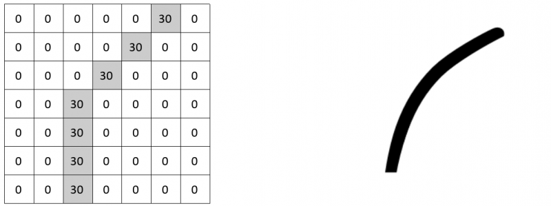
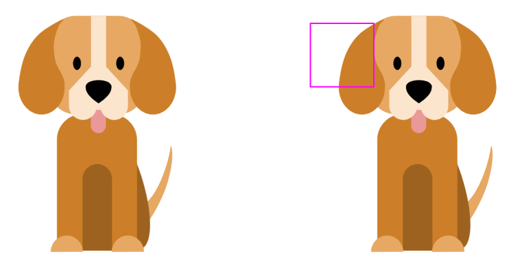
The filter has a pixel structure where high values correlate with the shape of the curve. The image of the dog below is used as an example. The filter is placed in the upper left corner.

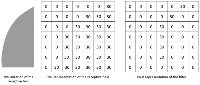
As the filter moves or strides over the input image, the filter values are multiplied by the original pixel values of the image and then added to obtain a single number. This process is repeated for each location on the image to obtain a single number for each unique location. When the filter scans each location of the image, an array of numbers is created: an activation map or feature map. This activation map identifies areas of the image in which a particular feature was present. A similar process can be performed with a filter designed to find semicircles to properly characterize all characteristics of an “ear”.

We have to go deeper

A traditional CNN contains “extra” layers that alternate between the convolution layers. First, dimension retention (Pool-layers) help to improve the robustness of the network, reduce the amount of free parameters in the network and therefore control overfitting by downsampling/aggregating information. ReLU activation functions are included to introduce non-linearities and finally fully connected layers are typically introduced as the last layer. This layer acts as a traditional classifier that uses the extracted high levels features as input. A classical CNN architecture would look like this:

Input → Conv → ReLU → Conv → ReLU → Pool → ReLU → Conv → ReLU → Pool → Fully Connected

In order to predict whether an image is a dog or a cat, the network must be able to recognize important features such as whiskers, pointed or drooping ears, different fur types, etc. That is why the network needs multiple convolution layers. The deeper into the network, the greater the number of passed convolution layers and therefore more complex features appear. These features can be semi-circles (combination of a curve and a straight edge) or squares (combination of several straight edges).

The fully-connected layer is located at the end of the network. This layer produces an N-dimensional vector where N stands for the number of classes (two in the case of the cat/dog classification). Each number in this N-dimensional vector represents the probability of a certain class.

A fully connected layer looks at the output of the previous layer and uses the features to decide the class. If the network predicts that an image is a dog, it will have high values ​​in the activation maps that represent important features such as hanging ears, 4 legs or a round nose, etc.

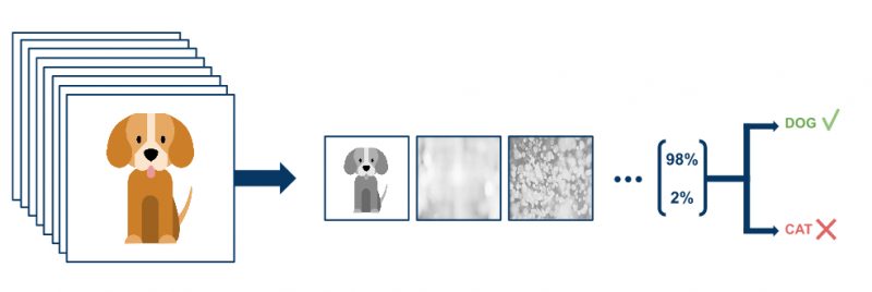
Success requires data

Multiple images must be fed to the network to find out if the network works. The output is compared with the ground truth to measure the success of the network. The key to this success is data. The more training data available to feed the network, the more training iterations can be performed and the more weights can be updated, resulting in a better-tuned network. Of course, there is more to it, important concepts such as hyperparameter tuning, network architecture, batch normalization, dropout, data augmentation are not discussed.